The price mechanism
What's on the page
The 'price mechanism' refers to how the free market forces of demand and supply interact to allocate scarce resources to the production of goods and services.
The process was first described by 18th Century Scottish philosopher and economist, Adam Smith, who saw the price mechanism as an 'invisible hand' where producers - acting in their own self-interest - [1] allocate scarce resources in a publicly beneficial way, satisfying wants and needs. Prices are seen as 'guiding' supply to meet demand.
The 'neo-classical' economists of the 19th Century, including English economist Alfred Marshall, added considerable detail to how the price mechanism works.
Markets, demand and supply
The price mechanism involves the forces of consumer demand and producer supply interacting in markets to allocate scarce resources.
Markets
Markets are arrangements between buyers and sellers to agree a price, a quantity to be supplied, and a time for payment and delivery.
We commonly think of markets as agreeing all of these 'on the spot' - in other words, for payment and delivery immediately. As well as spot markets there are also futures markets, where some element of the agreement is 'placed' into a future time period. Most commodity markets involve future agreements - given that the commodity might not exist at the time of the agreement.
Markets exist for all scarce resources, including markets for factors of production - factor markets - markets for goods and services - and financial markets, such as money and capital markets.
Effective demand and supply
When consumers are both willing and able to express their desires by entering a market, the result is 'effective demand' - that is, the desire to consume backed-up with an ability to pay - a purchasing power - namely, an income or budget.
When producers are both willing and able to enter a market, and supply, the result is 'effective supply' - that is, desire to supply backed-up with the ability to supply.
Analysis of demand and supply
An individual's demand refers to their willingness and ability to purchase goods and services at particular prices, and thereby satisfy their want's and needs. 'Market' demand refers to the sum of all individual demand at various prices.
The determinants of demand
Consumer demand is influenced by price, and a range of non-price factors.
Demand and price
The economist models demand by, firstly, holding all possible factors constant, and then varying the factor - or determinant - under consideration. The starting point for the model of demand (and supply) is the price of a good or service. The quantity demanded at various prices can be mapped using a demand schedule.
Price and quantity demanded are usually inversely related - at lower prices consumers will consume more.
Example
The following market demand schedule shows how the quantity demanded for bottled water varies over a range of hypothetical prices (expressed in $'s). A demand curve is derived from the schedule.

Given that the relationship between quantity demanded and price is inverse, a demand curve is, typically, downward sloping. There are several explanations of the downward slope of a demand curve:
Diminishing marginal utility
The principle of diminishing marginal utility suggests that marginal utility, or benefit, declines as more of a good is consumed - this means that a lower price is necessary to encourage demand. ‘Marginal’ is an important concept in economics and means the ‘additional’ amount of something resulting from an economic action – in this case, marginal utility is the additional benefit gained from consuming one more unit of a good or service.
In the example, the consumer is happy to pay a relatively high price for fewer units consumed, given that most utility is derived from the earliest units consumed. In the case of bottled water, thirst will be substantially satisfied by drinking the first bottle - in our example, a consumer is prepared to pay $3.00 for the first bottle consumed, and only $.2.50 for the second.
At higher quantities the consumer expects the marginal benefit of extra units to be less than before, and will therefore expect the price to be lower for these additional units. In simple terms, the consumer will expect the ratio of marginal utility and price to be the same for all goods consumed, so if a good rises in price marginal utility will be adjusted by consuming less [the 'equi-marginal' principle of consumer equilibrium].
Consumer equilibrium
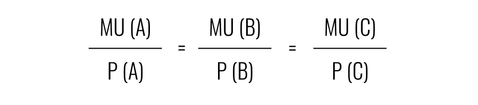
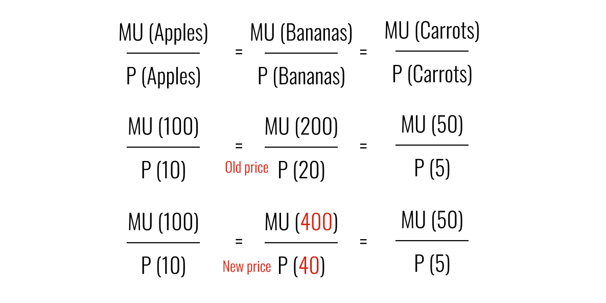
Hence, if a consumer spends all their income on just three goods, Apples (A), Bananas (B) and Carrots (C) they will be 'in equilibrium' when the ratio of marginal utility (MU) to price (P) will be equal - as we can see, the ratio is MU10/P1.
If the price of good B (Bananas) rises from its current level of 20 to 40, then the individual is pushed into a disequilibrium state. The obvious way to address this it is to 'increase' the level of MU to 400 to re-establish the 10/1 ratio. This can only be achieved by consuming less (given the underlying principle of diminishing marginal utility.)


Demand can also be explained in two other ways.
Income and substitution effect
If budgets are fixed, a lower price means more can be consumed - providing more ‘real’ income. For example, if a consumer has a budget of $2400, then at a price of $6 (at point A) he or she can buy 400 units of good X. If the price falls to $2, then the consumer can purchase 1200 units.
In a similar way, if prices of substitutes to good X are constant, a lower price of good X will encourage consumers to switch to good X.
In most cases, the income and substitution effect combine to create the negative price/demand relationship.
The two effects are called the ‘income effect’ and ‘substitution’ effect.

Non-price determinants of demand
Demand for specific goods and services is also determined by several 'non-price' determinants. Whenever a non-price determinant changes the demand curve which shift its position.
Comparative statics
The demand and supply model used by economists is an example of a comparative static model. This means that economists can compare two different static points - before an 'exogenous' (external) variable is changed, and then after it has changed.
For example, we can compare the equilibrium position (price and quantity) for raw coffee beans before a severe frost in Brazil - a major coffee growing region - and after the frost. The frost has increased production costs for coffee growers.
Using comparative statics means holding the 'endogenous' (internal) constant - in this case, price is the endogenous variable, and this is held constant. The exogenous variables are commonly referred to as 'non-price determinants'.
Non-price determinants include:
- Consumer incomes
- Tastes, trends, fashion and preferences
- Prices of substitute products
- Price of complementary products
- Expectations
If any of these non-price determinants change, the position of the demand curve will change. See below
Analysis of supply
Supply is the willingness and ability of firms to produce and take their goods and services to market. We can map the relationship between supply, price and other variables using supply schedules which can be visualised through supply curves.
A supply curve, typically, slopes up from left to right.
Price and the quantity supplied are positively related. At higher prices producers will supply more.
Supply schedule
A supply schedule lays out what firms plan to supply over a range of prices.

Supply curve
A supply curve can be derived from a supply schedule, and will tend to slope up from left to right.

Explanations of the upward slope
There are several explanations of why price and quantity supply are positively related, including:
Expectations of increased revenue
Higher prices encourage output because there is the expectation of higher revenue, which is price times quantity, and higher profit.

Of course, in reality this may not be the case as it depends on what is happening to other supply factors, and to demand. This reminds us that decisions to supply with respect just to price are 'hypothetical' - if all other factors remain constant (the ceteris paribus rule) then higher price will encourage more output as a result of its effect on expectations of profit.
We can see below that as price rises revenue (which is price times quantity) will also rise.

Increasing marginal cost
The marginal returns from adding more inputs to create more output tends to diminish. This means that (assuming factor inputs receive the same reward) the marginal cost of using more factors starts to increase. In this case, the firm will only be encouraged to increase output if the price of each unit increase.

If we combine these two theories we get a convincing explanation of why firms will be prepared to supply more at a higher price.
Changes in underlying determinants - shifts in demand
A change in the position of a demand curve indicates a change in the 'underlying determinants' of demand rather than a change in price.
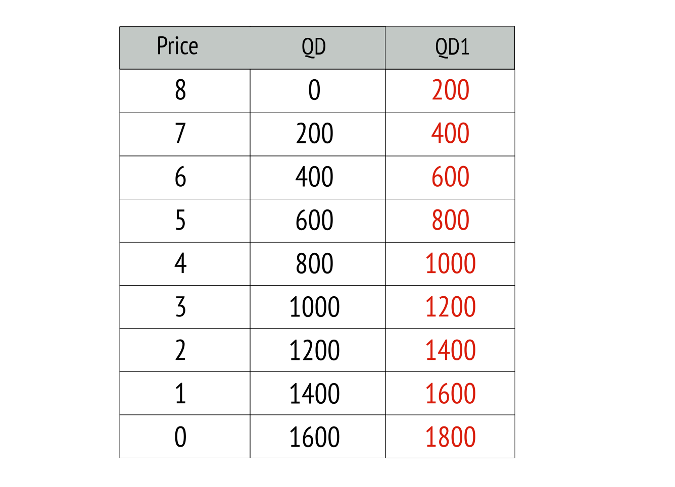
A demand curve can shift to the right (at D1) - an increase - or to the left (at D2) - a decrease following a change in an underlying determinant of demand. With an increase, more goods are demanded at all prices.
Increase in demand - shift to the right
The schedule and curve show that demand has increased by 200 units at each and every price.

Decrease in demand - shift to the left
The schedule and curve show that demand has decreased by 200 units at each and every price.


Several factors can cause a shift in a demand curve, including:
- Changes in income - which can affect consumer demand in two fundamental ways. In the case of normal goods, income and demand are positively related - an increase in income increases demand, and a reduction in income reduces demand. However, in the case of inferior goods, the relationship between income and demand is inverse - an increase in income reduces demand and a reduction in income increases demand. For example, as income rises individuals are likely to consume more 'luxury' (normal) goods and less basic (inferior) necessities.
- Changes in the price of substitutes will also affect demand, with a fall in the price of a substitute leading to a shift of demand to the left, and a rise in the price of a substitute causing demand to shift to the right.
- Changes in the price of related products, such as complements, will also shift the demand curve. For example, a rise in the price air travel may lead to a fall in the demand for overseas holidays.
- Changes in consumer's tastes and preferences will also affect demand. The demand for gym memberships has increased as more people to improve their levels of health.
- Changes in consumer expectations about the probability of an event, or regarding the need to purchase a good or service at some point in the future. For example, having heard that the price of a product is likely to increase in the future a consumer might alter there current consumption and make the purchase 'today' rather than wait. Consumers may speculate about price changes in the future and alter there current consumption. This is especially true in terms of the demand for financial securities, and exchange rates.
- Demand can also be influence by changes in the nature of the population - such as when a population ages - and changes in natural factors, such as changes in weather causing changes in the type of clothing demanded.
Shifts in supply
A shift of a supply curve is caused by a change in an underlying condition of supply, such as the cost of raw materials, rather than the price of the good or service.
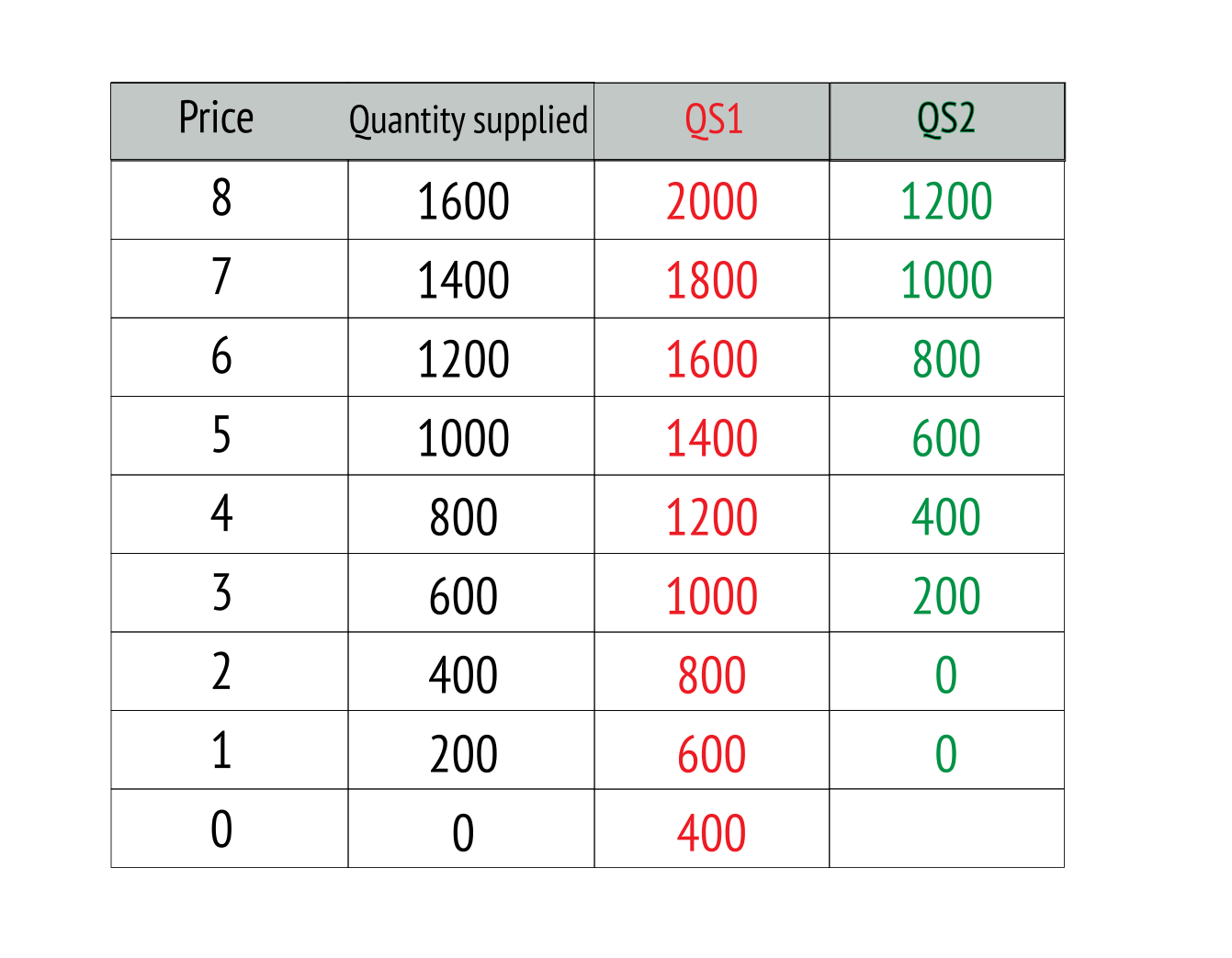
The following supply schedule shows the original supply against price, with two further columns - S1 indicates an increase in supply of 400 units at each price, and S2 indicates a reduction in supply of 400 units.
A shift of supply to the right
Taking data from the supply schedule we can identify S1 as an increase in supply - where the supply curve shifts to the right.

Assuming price is constant, a shift to the right (at S1) is an increase in supply which could be caused by;
- More available raw materials;
- An increase in the supply of labour;
- Subsidies on goods or services;
- A reduction in taxes;
- Unusually good weather or other beneficial supply factors.
A shift to the left in supply

A shift of a supply curve to the left (at S2) is a decrease in supply. Assuming the price is constant, a shift in supply to the left could be caused by:
- Less available raw materials;
- More expensive raw materials;
- A reduction in the supply of labour;
- Taxes on goods or services;
- Bad weather or other disruptive natural events.
[1] Smith, A - An Inquiry into the Nature and Causes of the Wealth of Nations (1776)